1 Introduction to R and RStudio
- Create and save files in RStudio
- Use R as a calculator
- Create first objects in R
- Call first functions in R
- Do you very first plot
This chapter introduces you to R and RStudio which you’ll be using throughout the course both to learn statistical concepts and to analyse real data. Often, R and RStudio are confused. However, they are not the same: R is the name of the programming language itself and RStudio is a so-called integrated development interface (IDE), a development environment that will make your life easier.
1.1 What is ?
R is a programming language for data analysis and statistical modelling. It is free (open-source software) and belongs, together with Python, to the most popular programming languages for data analysis. R has been introduced by Ross Ihaka and Robert Gentleman in 1996 (Ihaka and Gentleman 1996). It has many additional packages, which extend its functionality.
You can and should install R on your computer through the official R webpage. A short installation instruction with a list of packages for this course can be found on ILIAS. Additionally, you can refer to Ismay and Kim (2021), Chapter 1. You will find packages on R’s official webpage under CRAN (The Comprehensive R Archive Network). Not all packages are released through CRAN. However, in the beginning it is a good idea to use CRAN to find and install packages.
Packages are sometimes organized in topics, which you can explore via the CRAN Task Views. For environmental statistics, the following topics are relevant:
- Environmetrics: analysis of environmental data
- Multivariate: multivariate statistics
- Spatial: analysis of spatial data
- TimeSeries: time series analysis.
1.2 What is RStudio?
RStudio Desktop is an IDE for R (and some other languages). You can download and install the open-source version for your computer here. The RStudio interface is split in four main areas (Figure 1.1).
On the top left, you will type your commands and your text. The focus of this course is on reproducible research, and we will start using R Markdown in the next session.
The panel on the bottom left is the console where R executes your commands. This is the proper R system. When you start RStudio, the standard R text will be displayed there to inform you about the R being open source, its version and some other useful things.
The panel in the upper right contains your workspace, i.e. the objects that you generated during your working session in R. Additionally, you will find the history of your commands there.
The panel in the bottom right will show your plots (in case you are working with simple scripts and not with RMarkdown files). The tab “Files” helps you to browse your files.
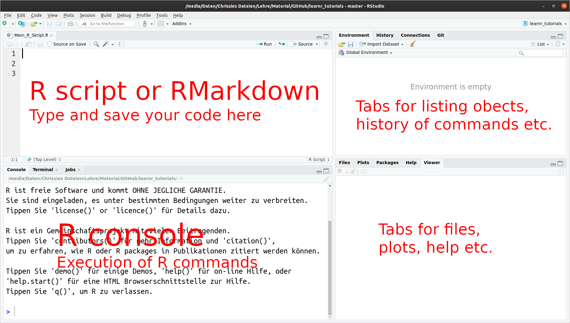
Figure 1.1: RStudio interface
1.3 Organize your work
To better organize your files, create a subfolders for data, scripts and notebooks in your main folder.
1.4 Practice on your own!
We will start the exercises C.1.1 and C.1.2 in class. Finish the exercises on your own and produce your first plot in exercise C.1.3 😄. If you need to type comments or answer with text, don’t forget to use the comment sign # at the beginning of each text line. Otherwise, R will misinterpret your text as commands and will try to execute them.
Remember to save your R script regularly! Click the save button in the upper left-hand corner of the window or hit Stg+s.
1.5 Turning in your work
- Save your R script as *.R file.
- Upload your *.R file to ILIAS. You will find an upload option in today’s session.
- You should receive a solution file after the upload.
Be sure to upload before the deadline!
1.6 Reading assignment
Chapters 1.1 and 1.2 in Ismay and Kim (2021)