3 What is data?
- Install an R package
- Load an installed data set
- Explore a data set and recognize the type of its variables
Data can be anything 😄. Usually, we will store data in a rectangular form, i.e. variables in columns and observations in rows. There are two dedicated object formats to store data, namely data.frame() and tibble(). They have both similar characteristics, however, the tibble is considered the modern form of a data frame and offers some advantages (details later).
In this chapter, we will have a look at a data set called palmerpenguins. It is provided in a dedicated package, so let’s install this package first.
3.1 Installing R packages
Packages that are available on the official CRAN (Comprehensive R Archive Network) can be installed with function install.packages('name_of_the_package'). It is important to provide the name of the package in quotes (single or double).
install.packages('palmerpenguins')To load a package, use the function library(name_of_the_package), this time without quotes!
3.2 Welcome the penguins!
Figure 3.1: Artwork by @allison_horst
The package has a dedicated website that is really worth visiting. The package contains two data sets, we will explore the shorter one, called penguins. To load a data set installed with a package, use the function data("name_of_data_set"). Be sure to put the name of the data set in quotes (single or double).
data("penguins")Let’s have a look at the object penguins.
penguins## # A tibble: 344 × 8
## species island bill_length_mm bill_depth_mm flipper_length_mm body_mass_g
## <fct> <fct> <dbl> <dbl> <int> <int>
## 1 Adelie Torgersen 39.1 18.7 181 3750
## 2 Adelie Torgersen 39.5 17.4 186 3800
## 3 Adelie Torgersen 40.3 18 195 3250
## 4 Adelie Torgersen NA NA NA NA
## 5 Adelie Torgersen 36.7 19.3 193 3450
## 6 Adelie Torgersen 39.3 20.6 190 3650
## 7 Adelie Torgersen 38.9 17.8 181 3625
## 8 Adelie Torgersen 39.2 19.6 195 4675
## 9 Adelie Torgersen 34.1 18.1 193 3475
## 10 Adelie Torgersen 42 20.2 190 4250
## # ℹ 334 more rows
## # ℹ 2 more variables: sex <fct>, year <int>This object is a tibble and contains a data set with 344 rows and 8 columns, meaning we have 8 variables measured on 344 animals. The first column contains the variable species that, you guessed it, shows the species of the animal. This variable is a so-called factor (indicated by <fct> below species). It means, it contains categorical information and has a certain number (usually a small one) of distinct values called levels. The levels in this case are
levels(penguins$species)## [1] "Adelie" "Chinstrap" "Gentoo"The above code uses the $ sign to access a whole column (i.e. variable) in the data set. This is very handy and an alternative to the square bracket method. The syntax is name_of_data_set$name_of_variable.
There are also numerical variables in the tibble. A numerical variable can be continuous, e.g. bill_length_mm (indicated by <dbl> meaning double), meaning that it contains decimal numbers or discrete, e.g. year (indicated by <int> meaning integer), meaning that it contains integers (whole numbers).
To summarize the data set, we can use the function summary().
summary(penguins)## species island bill_length_mm bill_depth_mm
## Adelie :152 Biscoe :168 Min. :32.10 Min. :13.10
## Chinstrap: 68 Dream :124 1st Qu.:39.23 1st Qu.:15.60
## Gentoo :124 Torgersen: 52 Median :44.45 Median :17.30
## Mean :43.92 Mean :17.15
## 3rd Qu.:48.50 3rd Qu.:18.70
## Max. :59.60 Max. :21.50
## NA's :2 NA's :2
## flipper_length_mm body_mass_g sex year
## Min. :172.0 Min. :2700 female:165 Min. :2007
## 1st Qu.:190.0 1st Qu.:3550 male :168 1st Qu.:2007
## Median :197.0 Median :4050 NA's : 11 Median :2008
## Mean :200.9 Mean :4202 Mean :2008
## 3rd Qu.:213.0 3rd Qu.:4750 3rd Qu.:2009
## Max. :231.0 Max. :6300 Max. :2009
## NA's :2 NA's :23.3 The square braces revisited
You already know how to access a certain position inside a vector. A tibble is a tow-dimensional object, it has rows and columns. To access a particular measurement, you need to provide both, its row and its column index. The following code picks the value in the first row and third column:
penguins[1, 3]## # A tibble: 1 × 1
## bill_length_mm
## <dbl>
## 1 39.13.4 Let’s look at them
We will talk much more about data visualization later. For now, just use the code below to visualize the relationship between the flipper length and the body mass of the animals.
library(ggplot2)

ggplot(data = penguins, mapping = aes(x = flipper_length_mm, y = body_mass_g, col = species)) +
  geom_point() +
  xlab('Flipper length (mm)') +
  ylab('Body mass (g)')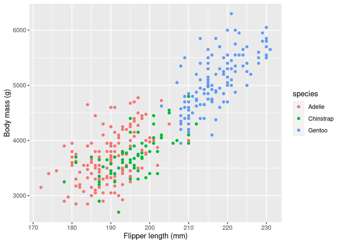
3.5 Practice on your own!
How many categorical and how many numerical variables are there? Consult help.
How many Gentoo penguins are present in the data set?
What is the time span of the measurements?
Find the levels of the variable
island.This is a challenge 🤓. Take the code that produced the visualization of flipper length and the body mass of the animals. Make an educated guess how to change the code such that it produces the visualization of the bill depth vs. body mass. Can you also guess how to adjust the label on the \(x\)-axis?
3.6 Reading assignment
Chapter 1.3 in Ismay and Kim (2021).
3.7 Turning in your work
- Save your R Notebook as an *.Rmd file.
- Upload your R Notebook to ILIAS. You don’t need to upload the .nb.html file. You will find an upload option in today’s session.
- You should receive a solution file after your upload. Be sure to upload before the deadline!
3.8 Additional reading
In case you prefer flights to penguins, you can have a look at data exploration in Chapter 1.4 in Ismay and Kim (2021)