10 Inference in linear regression
- Calculate confidence intervals for model parameters
- Interpret the summary of a linear regression model
- Use bootstrap for confidence intervals
In the last chapter, we learned how to fit a simple linear model. Remember the assumptions of the model:
- Linear relationship between variables
- Independence of residuals
- Normal residuals
- Equality of variance (called homoscedasticity) and a mean of zero in residuals
In this chapter, we will see how to judge the quality of our model. And we will learn what to do in case the normality and homoscedasticity assumptions are violated.
10.1 How good is the model?
The data that we model have a certain variability that we quantify by e.g. its variance. To judge how good a model captures the relationship between the dependent variable and the predictors, we could quantify how much variability of the dependent variable can be explained by the model. Thus, we split the variability of the dependent variable (i.e. our observed data) as:
\[ \begin{align*} \mathit{SQT} &= \mathit{SQE} + \mathit{SQR}\\ \sum^{n}_{i = 1} (y_i-\bar{y})^2 &= \sum^{n}_{i=1} (\hat{y}_i - \bar{y})^2 + \sum^{n}_{i=1} (y_i - \hat{y}_i)^2\\ \end{align*} \]
where \(y_i\): observed data, \(\bar{y}\): mean, \(\hat{y}_i\): fitted values
- \(\mathit{SQT}\) Sum of squares total: variability or variance of the data
- \(\mathit{SQE}\) Sum of squares explained: variability explained by the model
- \(\mathit{SQR}\) Sum of squares residual: variability not explained by the model
The \(\mathit{SQE}\) quantifies the variability of the fitted values around the mean of the data and \(\mathit{SQR}\) shows how much variability the model fails to capture. The smaller this residual variability \(\mathit{SQR}\) the better the model! The so-called coefficient of determination calculates the proportion of explained variability. The larger it is the better the model 😄:
\[R^2 = \frac{\mathit{SQE}}{\mathit{SQT}} = 1 - \frac{SQR}{SQT} = 1- \frac{\sum^{n}_{i=1} (y_i - \hat{y}_i)^2}{\sum^{n}_{i = 1} (y_i - \bar{y}_i)^2}\]
Let’s go back to our example and look at the coefficient of determination.
lin_mod <- lm(formula = time_lib ~ travel_time, data = survey)

get_regression_summaries(lin_mod) %>% kable()| r_squared | adj_r_squared | mse | rmse | sigma | statistic | p_value | df | nobs |
|---|---|---|---|---|---|---|---|---|
| 0.532 | 0.529 | 430.4021 | 20.74614 | 20.851 | 224.697 | 0 | 1 | 200 |
There is a lot of information coming with the summary. In details, we find:
-
r_squared: Coefficient of determination \(R^2\) -
adj_r_squared: \(R^2_\text{ajd} = 1 - (1 - R^2) \frac{n-1}{n - p - 1}\), \(n\): number of data points, \(p\): number of predictors (without the intercept); more robust than \(R^2\) for multiple linear regression -
mse: mean standard errormean(residuals(lin_mod)^2) -
rmse: square root ofmse -
simga: standard error of the error term \(\varepsilon\) -
statistic: value of the \(F\) statistics for the hypothesis test, where \(H_0\): all model parameters equal zero -
p-value: \(p\) value of the hypothesis test -
df: degrees of freedom, here number of predictors -
nobst: number of data points
Thus, we conclude hat our model explained 53% of the variance in the data.
10.2 Bootstrap with infer: Confidence interval for the slope
In case, the residuals are non-normally distributed and/or heteroscedastic, the confidence intervals for the model parameters could be wrong. In particular for small data sets, the violation of those assumptions is problematic. To avoid interpreting (possibly) wrong confidence intervals, we can use the bootstrap to construct confidence intervals that do not require the normality and homoscedasticity of residuals. However, they still require independent data (this is always the case for the ordinary bootstrap).
In a simple linear regression, the most interesting parameter is the slope. We can use our usual framework in infer to determine its confidence interval.
Step 1: Bootstrap the data and calculate the statistic slope
bootstrap_distn_slope <- survey %>%
  specify(formula = time_lib ~ travel_time) %>%
  generate(reps = 10000, type = "bootstrap") %>%
  calculate(stat = "slope")
Step 2: Calculate the confidence interval
percentile_ci <- bootstrap_distn_slope %>%
  get_confidence_interval(type = "percentile", level = 0.95)

percentile_ci
## # A tibble: 1 × 2
## lower_ci upper_ci
## <dbl> <dbl>
## 1 -0.848 -0.687Step 3: Visualise the result
visualize(bootstrap_distn_slope) +
shade_confidence_interval(endpoints = percentile_ci) 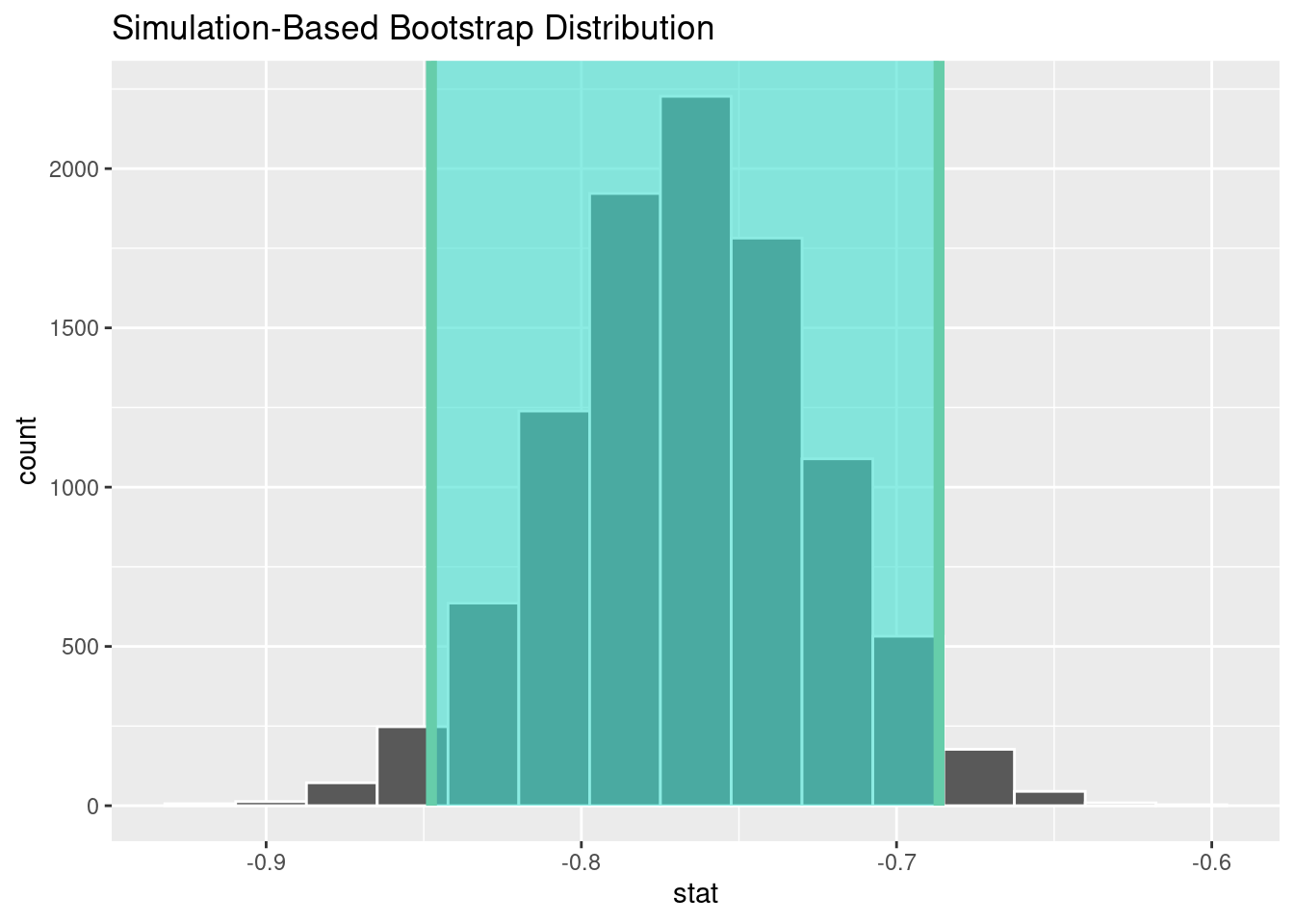
Compared to the standard confidence interval based on the normality and homoscedasticity assumptions, the bootstrap confidence interval is similar.
get_regression_table(lin_mod) %>%
filter(term == 'travel_time') %>%
kable()| term | estimate | std_error | statistic | p_value | lower_ci | upper_ci |
|---|---|---|---|---|---|---|
| travel_time | -0.766 | 0.051 | -14.99 | 0 | -0.867 | -0.665 |
This is because in our model, the assumptions were valid. In such a case, the confidence intervals are similar and you can safely use the standard confidence interval. Otherwise prefer the bootstrap.
10.3 Practice on your own!
- You will analyse the relationship between the number of plant species and the number of endemic species on the Galapagos islands. The data set is called
galaand is part of the libraryfaraway.- Load the data set and read the help pages to understand the meaning of the variables.
- We want to know how the number of endemic species depends on the number of plant species on the islands. Fit a linear regression model that takes the number of species as predictor and the number of endemic species as dependent variable.
- Check the model assumptions.
- Use the workflow in
inferto calculate a confidence interval for the slope in the model. - Compare the confidence interval based on normality assumption and the bootstrap confidence intervals
10.4 Reading assignment
Chapter 10 in Ismay and Kim (2021)