11 Introduction to time series analysis
11.1 What are time series?
Time series are sequences of values ordered by time. The order of the values is crucial. Often, subsequent values are similar to each other, i.e. correlated. This implies that many statistical techniques which require independent observations do not work.
11.2 An example from the German Meteorological Service (DWD)
We will analyse daily temperature and precipitation data. The goal is to see whether (i) we can detect a trend in the data and (ii) how the data fluctuates through the year. A trend is any long-term change in the data which is not due to obvious cyclic processes like the yearly fluctuation. In contrast, seasonality shows exactly this, a (more or less) regular fluctuation which repeats itself in a certain time.
I downloaded the data using the library
rdwd (https://bookdown.org/brry/rdwd/) on 20 June 2022. The data was measured daily at the station “Koeln-Bonn” starting from 1957 to end of 2021. You can find the complete data description here:
We will need the following variables:
| Variable | Description | Format/Unit |
|---|---|---|
MESS_DATUM |
the date of measurements | yyyymmdd |
TMK |
daily mean of temperature | °C |
RSK |
daily precipitation height | mm |
We load the necessary libraries.
rdwddownloads a zipped file. First, we need to unzip it and then to read it in. Note that the NAs are coded as “-999”. We store the results in a subfolder called data/Koeln-Bonn/.
unzip('data/daily_kl_historical_tageswerte_KL_02667_19570701_20211231_hist.zip', exdir = "data/Koeln-Bonn")


clim <- read_delim('data/Koeln-Bonn/produkt_klima_tag_19570701_20211231_02667.txt', delim = ';', na = '-999', trim_ws = TRUE)
## Rows: 23560 Columns: 19
## ── Column specification ────────────────────────────────────────────────────────
## Delimiter: ";"
## chr (1): eor
## dbl (18): STATIONS_ID, MESS_DATUM, QN_3, FX, FM, QN_4, RSK, RSKF, SDK, SHK_T...
##
## ℹ Use `spec()` to retrieve the full column specification for this data.
## ℹ Specify the column types or set `show_col_types = FALSE` to quiet this message.
clim## # A tibble: 23,560 × 19
## STATIONS_ID MESS_DATUM QN_3 FX FM QN_4 RSK RSKF SDK SHK_TAG
## <dbl> <dbl> <dbl> <dbl> <dbl> <dbl> <dbl> <dbl> <dbl> <dbl>
## 1 2667 19570701 5 16 2.9 NA NA NA NA NA
## 2 2667 19570702 5 4.7 1.8 NA NA NA NA NA
## 3 2667 19570703 5 10.3 3.5 NA NA NA NA NA
## 4 2667 19570704 5 9.6 3.4 NA NA NA NA NA
## 5 2667 19570705 5 10.4 2.9 NA NA NA NA NA
## 6 2667 19570706 5 9.2 2.9 NA NA NA NA NA
## 7 2667 19570707 5 10.5 3.5 NA NA NA NA NA
## 8 2667 19570708 5 15.9 2.2 NA NA NA NA NA
## 9 2667 19570709 5 13.2 3.1 NA NA NA NA NA
## 10 2667 19570710 5 18.2 2.6 NA NA NA NA NA
## # ℹ 23,550 more rows
## # ℹ 9 more variables: NM <dbl>, VPM <dbl>, PM <dbl>, TMK <dbl>, UPM <dbl>,
## # TXK <dbl>, TNK <dbl>, TGK <dbl>, eor <chr>The date of the measurement is not a proper date format and we must convert it first.
## # A tibble: 23,560 × 19
##    STATIONS_ID MESS_DATUM  QN_3    FX    FM  QN_4   RSK  RSKF   SDK SHK_TAG
##          <dbl> <date>     <dbl> <dbl> <dbl> <dbl> <dbl> <dbl> <dbl>   <dbl>
##  1        2667 1957-07-01     5  16     2.9    NA    NA    NA    NA      NA
##  2        2667 1957-07-02     5   4.7   1.8    NA    NA    NA    NA      NA
##  3        2667 1957-07-03     5  10.3   3.5    NA    NA    NA    NA      NA
##  4        2667 1957-07-04     5   9.6   3.4    NA    NA    NA    NA      NA
##  5        2667 1957-07-05     5  10.4   2.9    NA    NA    NA    NA      NA
##  6        2667 1957-07-06     5   9.2   2.9    NA    NA    NA    NA      NA
##  7        2667 1957-07-07     5  10.5   3.5    NA    NA    NA    NA      NA
##  8        2667 1957-07-08     5  15.9   2.2    NA    NA    NA    NA      NA
##  9        2667 1957-07-09     5  13.2   3.1    NA    NA    NA    NA      NA
## 10        2667 1957-07-10     5  18.2   2.6    NA    NA    NA    NA      NA
## # ℹ 23,550 more rows
## # ℹ 9 more variables: NM <dbl>, VPM <dbl>, PM <dbl>, TMK <dbl>, UPM <dbl>,
## #   TXK <dbl>, TNK <dbl>, TGK <dbl>, eor <chr>
We plot the temperature data.
ggplot(data = clim, aes(x = MESS_DATUM, y = TMK)) +
  geom_line() +
  labs(y = 'Daily mean temperature (°C)',
       x = 'Date')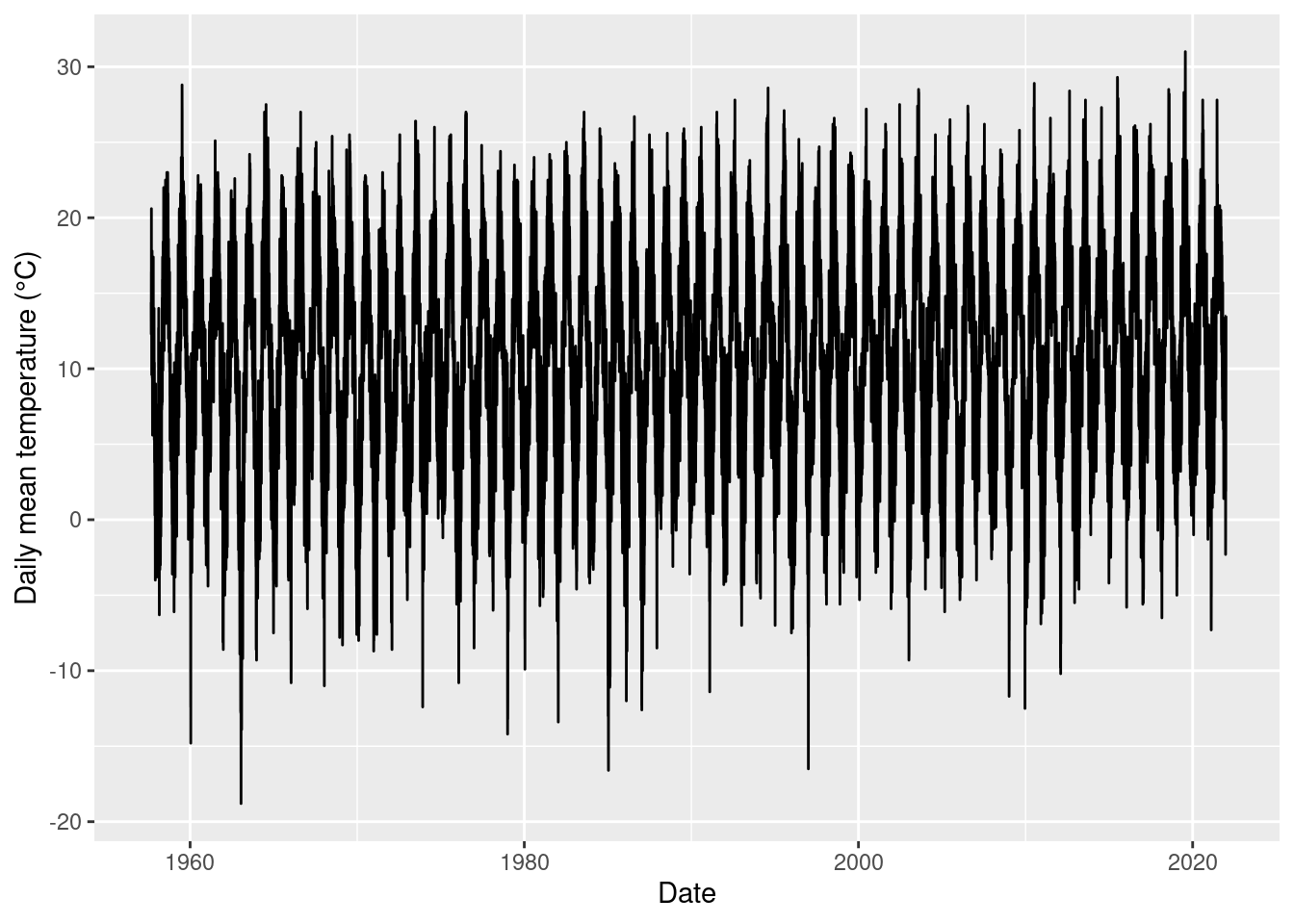
We want to analyse complete years only. Which years should be deleted because of too few data points?
## # A tibble: 65 × 2
##    `year(MESS_DATUM)`     n
##                 <dbl> <int>
##  1               1957   184
##  2               1958   365
##  3               1959   365
##  4               1960   366
##  5               1961   365
##  6               1962   365
##  7               1963   365
##  8               1964   366
##  9               1965   365
## 10               1966   365
## # ℹ 55 more rows
The year 1957 is incomplete and we exclude it.
11.3 Trend analysis of yearly data
We summarize the temperature to yearly values to exclude the seasonal fluctuations. This helps to analyse the trend.
temp_yearly <- clim %>%
  group_by(year(MESS_DATUM)) %>%
  summarize(mean_temp = mean(TMK, na.rm = T)) %>%
  rename(year = `year(MESS_DATUM)`)

temp_yearly
## # A tibble: 64 × 2
## year mean_temp
## <dbl> <dbl>
## 1 1958 9.76
## 2 1959 10.6
## 3 1960 10.1
## 4 1961 10.5
## 5 1962 8.56
## 6 1963 8.48
## 7 1964 9.86
## 8 1965 9.26
## 9 1966 10.2
## 10 1967 10.5
## # ℹ 54 more rowsPlot of yearly mean temperature data.
ggplot(temp_yearly, aes(x = year, y = mean_temp)) +
  geom_line() +
  geom_smooth(formula = 'y ~ x', method = 'loess', se = FALSE) +
  ylim(5, 15) +
  labs(y = 'Yearly mean temperature (°C)',
       x = 'Date')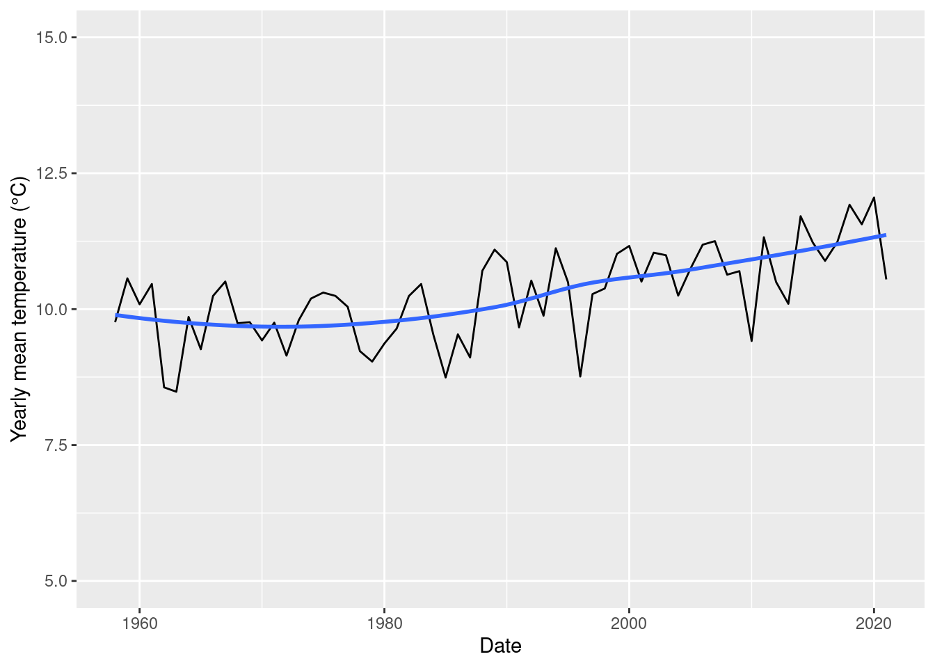
There seem to be an upward trend, but is it significant or due to chance. To answer this question we use the Mann-Kendall test for trend. The null and alternative hypothesis of the test are:
- \(H_0\): data does not have a trend.
- \(H_1\): data has a trend.
The test calculates a statistics called \(\tau\). It is based on a comparison of all possible pairs of variables and their succeeding neighbours. If \(\tau < 0\), then more neighbouring points are smaller, and the data has a negative trend. If \(\tau > 0\) more neighbouring points are larger, and the data has a positive trend. If \(\tau \approx 0\), then the smaller and larger neighbouring points are in balance, and there is no trend.
MannKendall(temp_yearly$mean_temp)## tau = 0.452, 2-sided pvalue =1.1921e-07The \(p\) value is small. It is plausible to conclude that there is a positive trend because \(\tau > 0\).
By how much did the mean temperature increase per year? We calculated differences of yearly temperature of consecutive years. We use the function reframe() instead of summarize(), because we don’t summarize the data based on groups, but because we calculate differences between years, which will decrease the number of rows. Check the help function for more information.
temp_diff <- temp_yearly %>%
  reframe(temp_diff = diff(mean_temp)) %>%
  mutate(year = temp_yearly$year[-1])

mean_diff <- temp_diff %>%
  summarise(mean = mean(temp_diff))
Plot the distribution of differences.
ggplot(temp_diff, aes(x = temp_diff)) +
  geom_histogram(bins = 15, col = 'white') +
  geom_vline(aes(xintercept = mean_diff$mean, color = "mean difference")) +
  labs(x = "Temperature difference (°C)", color = "Line")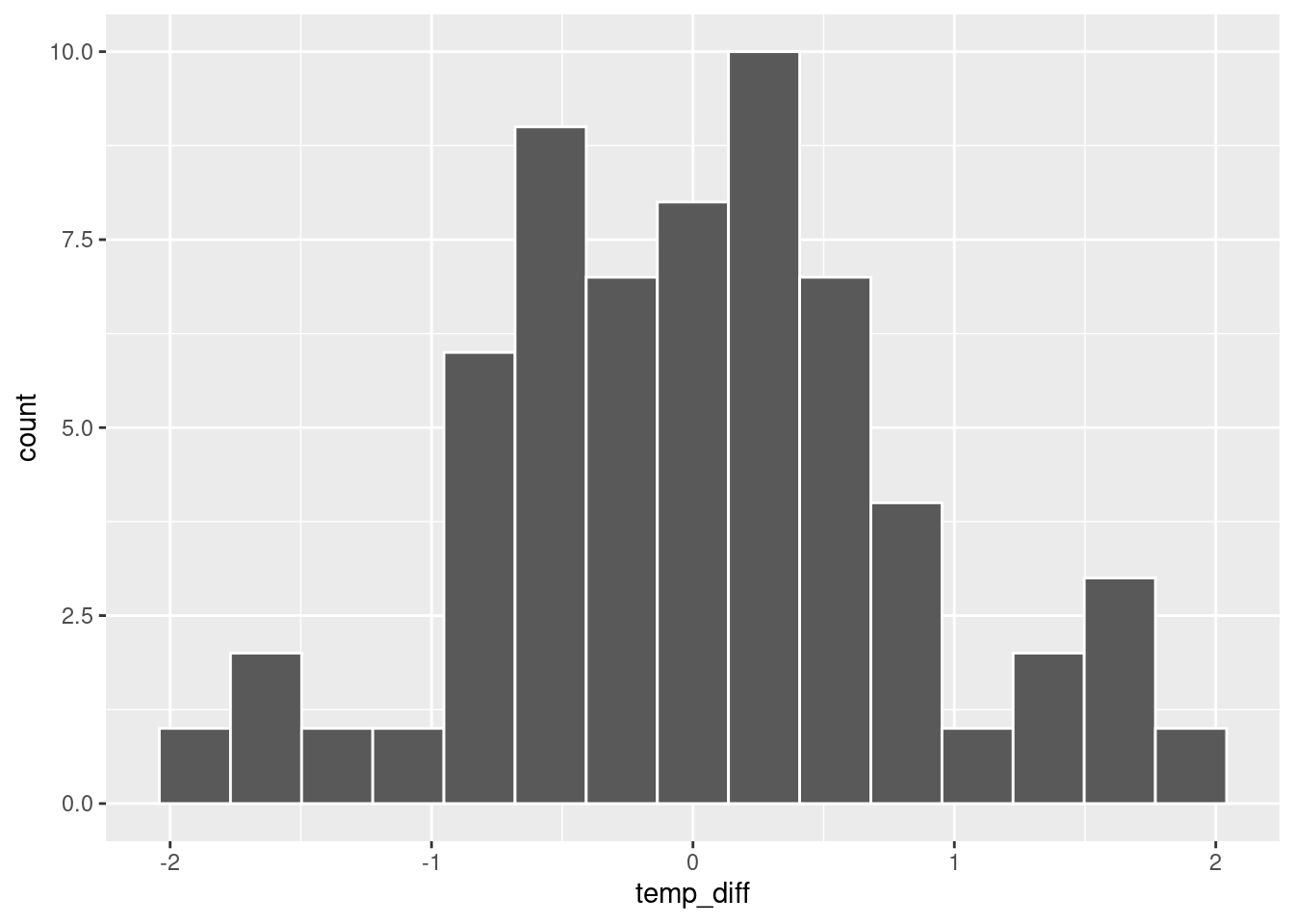
We see a mean increase of 0.01 degrees per year. For a robust estimate of the mean, with confidence interval, we could use bootstrapping.
11.4 Analysis of seasonality
Summarize by month
temp_monthly <- clim %>%
  group_by(year(MESS_DATUM), month(MESS_DATUM)) %>%
  summarize(mean_temp = mean(TMK, na.rm = T)) %>%
  rename(year = `year(MESS_DATUM)`, month = `month(MESS_DATUM)`) %>%
  mutate(date = ymd(paste(year, month, '15', sep = '-'))) %>%
  relocate(date)
## `summarise()` has grouped output by 'year(MESS_DATUM)'. You can override using
## the `.groups` argument.
temp_monthly## # A tibble: 768 × 4
## # Groups: year [64]
## date year month mean_temp
## <date> <dbl> <dbl> <dbl>
## 1 1958-01-15 1958 1 2.08
## 2 1958-02-15 1958 2 4.46
## 3 1958-03-15 1958 3 1.89
## 4 1958-04-15 1958 4 6.74
## 5 1958-05-15 1958 5 13.8
## 6 1958-06-15 1958 6 15.5
## 7 1958-07-15 1958 7 17.7
## 8 1958-08-15 1958 8 18.0
## 9 1958-09-15 1958 9 16.1
## 10 1958-10-15 1958 10 10.4
## # ℹ 758 more rowsPlot monthly values. The seasonality seems rather constant over time.
ggplot(temp_monthly, aes(x = date, y = mean_temp)) +
  geom_line() +
  labs(x = 'Date',
       y = 'Mean daily tempearture (°C)')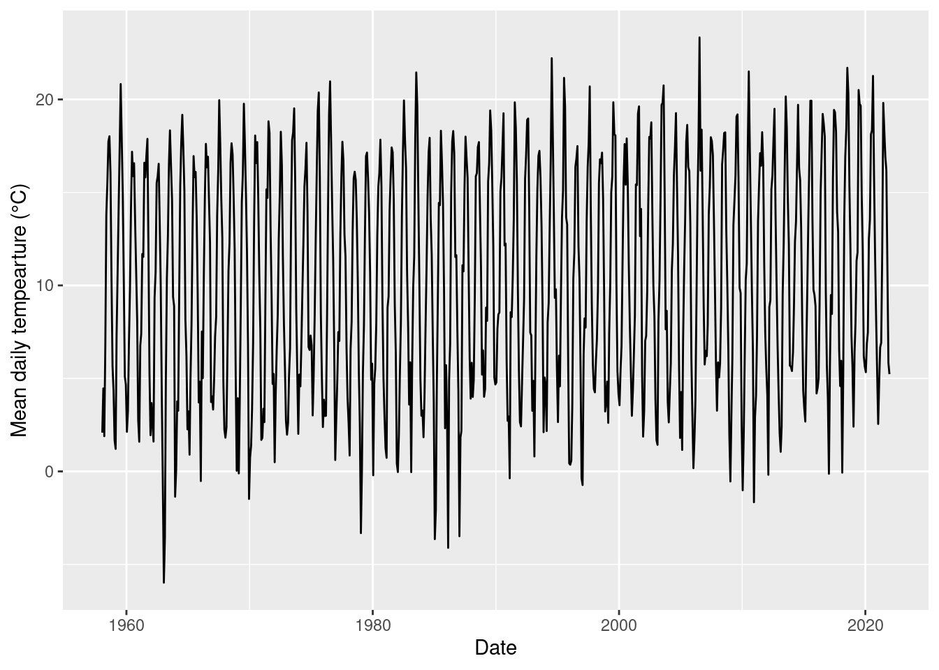
The overall seasonality.
ggplot(temp_monthly, aes(x = as_factor(month), y = mean_temp)) +
  geom_boxplot() +
  scale_x_discrete(labels = month.abb) +
  labs(x = 'Month',
       y = 'Variation of the mean yearly temperature (°C)')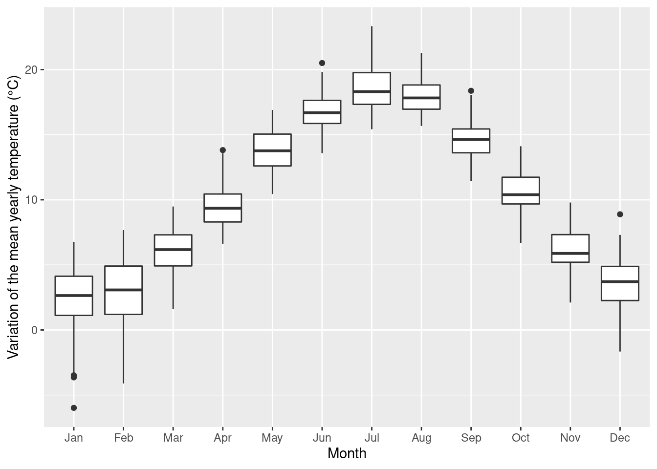
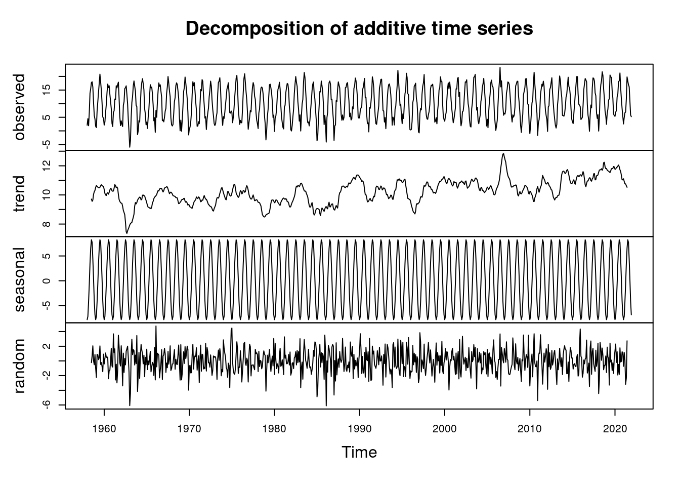
11.5 Advanced: Simultaneous analysis of trend and seasonality
We can use a model to decompose the time series into a trend, seasonality and a rest (remainder) component. This model is additive, meaning that when you sum the components, you get back your original time series. The model assumes that the seasonality remains stable over time, i.e. it is inappropriate for climate change studies. However, it is still a good starting point.
We need to convert the data to a ts (time series) object first. This type of objects keeps the data along with the time.
time_series <- ts(temp_monthly$mean_temp, start = c(1958, 1), end = c(2021, 12), frequency = 12)

str(time_series)
## Time-Series [1:768] from 1958 to 2022: 2.08 4.46 1.89 6.74 13.82 ...We use the function decompose() to decompose the time series.
Plot the trend using ggfortify. This library helps to transform the complicated object created by decompose() to a data.frame which can be easily plotted with ggplot().
ggplot(data = fortify(components), aes(x = Index, y = trend)) +
  geom_line() +
  annotate('rect', xmin = as.Date('2006-01-01'), xmax = as.Date('2007-12-31'), ymin = -Inf, ymax = Inf, fill = 'red', alpha = 1/3) +
  ylim(5, 15) +
  labs(x = 'Date',
       y = 'Trend component of the temperature (°C)',
       title = 'Red bar highlights the year 2007.')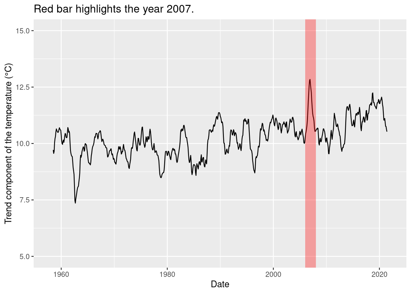
The large peak is due to the highest monthly mean in July 2007, don’t over-interpret this as a change in the trend!
General advice:
- If you want to analyse the trend, you need to get rid of the seasonality. The most simple way is to calculate yearly data (if not already provided) and then do the Mann-Kendall test to test for a trend.
- Calculate the mean change over years or analyse changes in more details. Report about those changes and the \(p\) value of the test.
- If you have seasonality, you can use
decompose()to decompose the data and estimate trend and seasonality. However, remember that the model assumes that the seasonality remains stable over time.
11.6 Practice on your own!
Select another location and repeat the analysis of temperature. Use the functions from the
rdwdlibrary (https://bookdown.org/brry/rdwd/).Analyse the precipitation data. Is there a trend? Instead of calculating mean values, you must sum the precipitations! Analyse the yearly sums only, no decomposition because seasonality is less important.