A Statistics refresher
- Refresh basic statistics
This chapter is a short refresher on the basic statistics and does not replace a statistics book. I will use the penguins data set to calculate the examples.
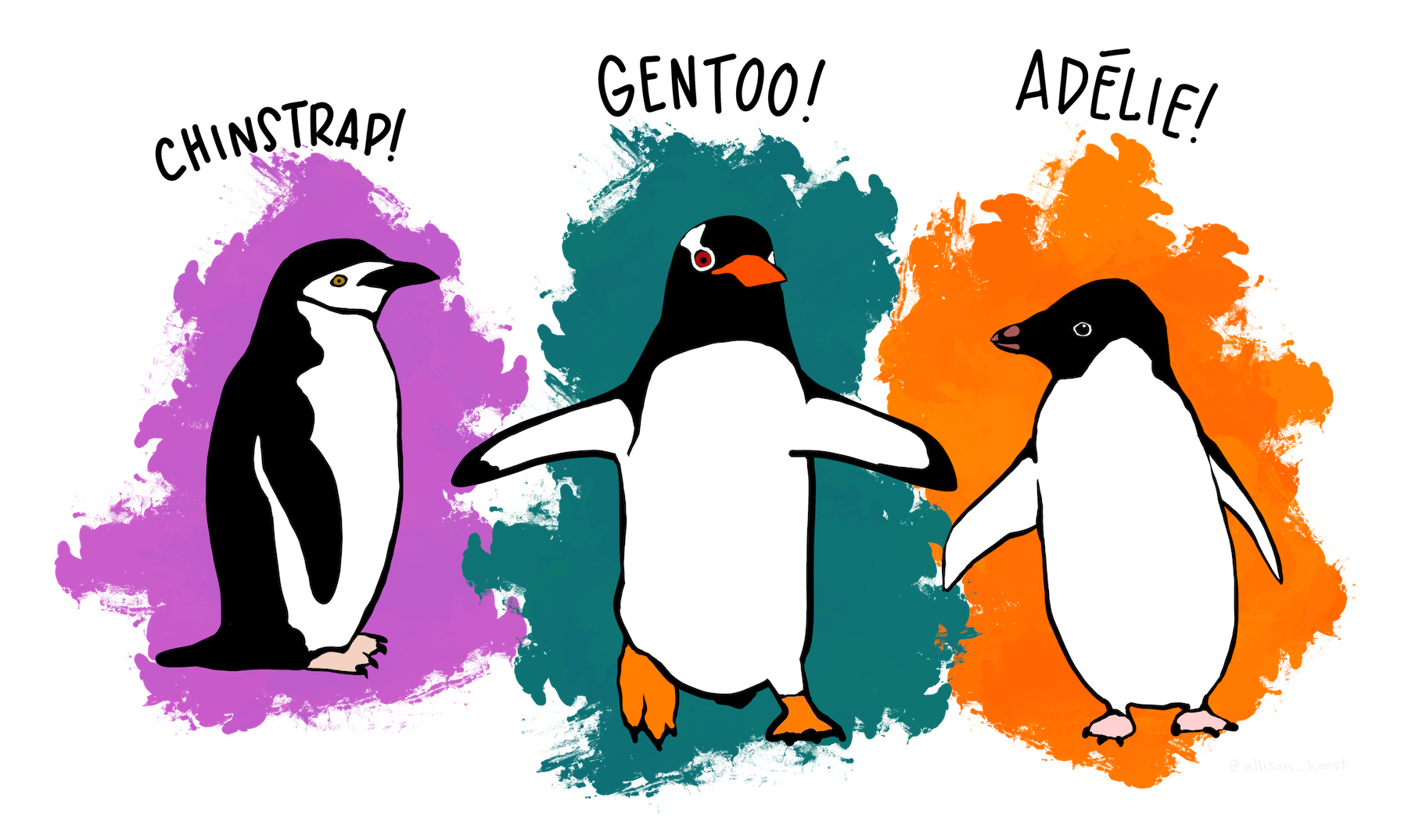
Figure A.1: Artwork by @allison_horst
A.1 Descriptive statistics
A.1.1 Mean
The mean is one of the common summary statistics you can calculate for your data. To calculate the mean you sum all the values in your data set and divide the sum by the number of values.
\[\bar{x} = \sum_{i = 1}^{i = n} \frac{x_i}{n}\] where:
- \(\bar{x}\): mean value of data set \(x\)
- \(i\): index running from 1 to \(n\), the number of your data (sample size)
- \(x_i\): single data points in the data sets \(x\)
A simple example first, before we turn to the penguins. Let’s calculate the mean of the data set a containing the values 2, 4.3, 5 and 10 by hand and compare it to the values obtained with the function mean().
## [1] 5.325
r_mean## [1] 5.325As expected, the values are identical. Let’s now calculate the mean bill length of the penguins.
mean(x = penguins$bill_length_mm)## [1] NAThe function mean() returns NA if there are missing values in the data set. Remember to exclude NAs with na.rm = TRUE to get a meaningful result.
mean(x = penguins$bill_length_mm, na.rm = TRUE)## [1] 43.92193A.1.2 Variance and standard deviation
Variance and standard deviation are both measures of variability in your data. They show how far the data deviates from its mean value on the average. This deviation is defined as the squared difference between a data point and the mean of the data. The variance is defined as:
\[v = \frac{1}{n-1} \sum_{i = 1}^{i = n} (x_i - \bar{x})^2\]
The standard deviation is the square root of the variance and is defined as:
\[s = \sqrt{\frac{1}{n-1} \sum_{i = 1}^{i = n} (x_i - \bar{x})^2}\] where:
- \(\bar{x}\): mean value of data set \(x\)
- \(i\): index running from 1 to \(n\), the number of your data points (sample size)
- \(x_i\): single data points in the data sets \(x\)
How large is the standard deviation in the data set a? Again, we compare the results of by-hand calculation and the output of the function sd().
sd_hand <- sqrt(((2 - r_mean)^2 + (4.3 - r_mean)^2 + (5 - r_mean)^2 + (10 - r_mean)^2)/(4 - 1))

r_sd <- sd(a)

sd_hand
## [1] 3.369842
r_sd## [1] 3.369842Again, identical 😄. How large is the standard deviation of penguins’ bill lengths? Don’t forget to exclude the missing values!
sd(x = penguins$bill_length_mm, na.rm = TRUE)## [1] 5.459584A.2 Measures of association
A.2.1 Linear correlation coefficent
Aka Pearson correlation coefficient and Pearson product-moment correlation coefficient measures the linear association between two numeric variables:
\[ r = \frac{\sum_{i = 1}^{i = n} (x_i - \bar{x})(y_i - \bar{y})}{ \sqrt{\sum_{i = 1}^{i = n} (x_i - \bar{x})^2} \sqrt{\sum_{i = 1}^{i = n} (y_i - \bar{y})^2}}\] where:
- \(\bar{x}\) and \(\bar{y}\): mean values of data set \(x\) and \(y\), respectively
- \(i\): index running from 1 to \(n\), the number of your data points (sample size)
- \(x_i\) and \(y_i\): single data points in the data sets \(x\) and \(y\), respectively
The Pearson correlation coefficients varies between -1 (perfect negative correlation) and 1 (perfect positive correlation). A value around zero shows no linear correlation. However, a different kind of assiciation might exist in the data. Remember to always plot your data!
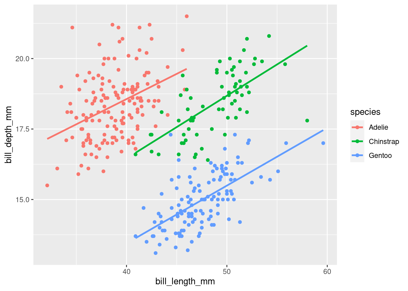
How large is the correlation coefficient between the bill length and the bill depth for the species Adélie?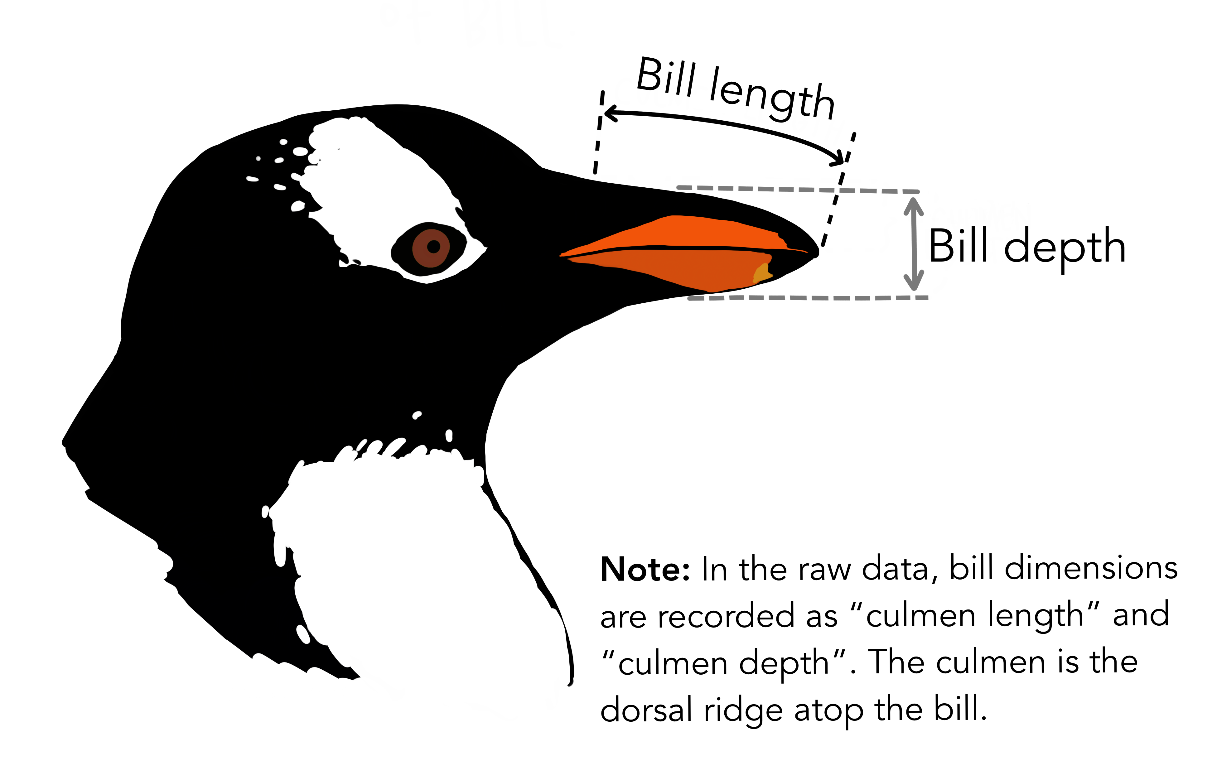
Figure A.2: Artwork by @allison_horst
adelie <- penguins %>%
  filter(species == 'Adelie')

cor(adelie$bill_length_mm, adelie$bill_depth_mm, method = 'pearson', use = 'pairwise.complete.obs')
## [1] 0.3914917We need to distinguish between species because the correlations differ between them.
penguins %>%
  group_by(species) %>%
  summarise(cor = cor(bill_length_mm, bill_depth_mm, method = 'pearson', use = 'pairwise.complete.obs'))
## # A tibble: 3 × 2
## species cor
## <fct> <dbl>
## 1 Adelie 0.391
## 2 Chinstrap 0.654
## 3 Gentoo 0.643
ggplot(data = penguins, aes(x = bill_length_mm, y = bill_depth_mm, col = species)) +
  geom_point() +
  geom_smooth(se = FALSE, method = lm)